
Liquidity Sentinel: Crypto Exchange Withdrawal & Solvency Model
A stress testing framework that models how much fiat a crypto exchange needs to survive a weekend withdrawal run — sized against OJK’s regulatory requirements and the realities of Indonesian banking infrastructure.
→ GitHub · Live Dashboard · Google Collab
// The problem Proof of Reserve does not solve
Proof of Reserve attestations show that an exchange holds crypto assets equal to or greater than user crypto balances. They are useful — but they leave three things unmeasured.
Fiat withdrawal capacity. PoR confirms the crypto side of the ledger. It does not tell you whether the exchange can process IDR withdrawals over a 64-hour weekend window when bank transfer rails are offline. In Indonesia, interbank settlement runs on SKN-BI and RTGS, they operate within defined service windows, until 2pm on weekdays. From Friday evening to Monday morning, an exchange cannot top up its fiat reserves from banking partners regardless of what is on its balance sheet. They can use BI-FAST and ONLINE but there is a limit of Rp250 million and Rp50 million respectively, which is very inconvenience. So, whatever fiat sat in the payment gateway when the weekend started is the best scenario for my fellow ops.
Asset quality under pressure. A static snapshot does not model what happens when withdrawal velocity doubles. Holding reserves in the exchange’s own native token — which FTX did with FTT — passes a PoR check and collapses under redemption pressure. The relevant question is not what is held but what survives the scenario.
Derivatives exposure. Spot-only exchanges should be 1:1 backed — PoR mostly covers this. Exchanges offering perpetual futures or CFD equity have an additional liability that PoR does not capture: when a user’s margin is insufficient to cover their loss, the exchange absorbs the deficit. In a violent market move with a liquidation cascade, this can exceed the insurance fund and become an exchange-level solvency problem.
This model builds the simulation layer that PoR does not provide.
// The Indonesian regulatory floor
Under POJK No. 27 of 2024, OJK has established a framework for licensed crypto exchanges (Pedagang Aset Keuangan Digital) that is more structurally prescriptive than most jurisdictions. Rather than leaving reserve policy to internal risk management, the regulation sets hard floors that the model treats as binding constraints — not aspirational targets.
The equity floor. A licensed Pedagang must maintain a minimum equity of Rp 50 billion at all times. This is the regulatory equivalent of what traditional securities firms call MKBD (Modal Kerja Bersih Disesuaikan), but simplified into a fixed threshold rather than a dynamic ratio. The model’s solvency assessment uses this floor as the hard lower bound: a scenario that breaches Rp 50 billion in equity is not merely unfavorable — it is a regulatory violation.
The 30/70 storage rule. A Pedagang may hold a maximum of 30% of total consumer-owned crypto assets in its own custody. The remaining 70% must be placed with a licensed Custodian (Pengelola Tempat Penyimpanan). Of the 30% retained internally, at least 70% must be in cold storage (offline), with a maximum of 30% in hot storage (online) for operational liquidity. This means the exchange’s readily accessible crypto liquidity — its hot wallet — is capped at 9% of total consumer assets (30% × 30%). The model uses this ceiling when computing liquidatable crypto buffers under stress.
The 100% fund segregation rule. All consumer fiat funds must be placed in separate accounts at the licensed Clearing and Settlement Institution (Lembaga Kliring Penjaminan dan Penyelesaian). The exchange is strictly prohibited from using these funds for its own operations. This matters for the model because it eliminates a common (and legally impermissible) workaround: an exchange cannot dip into pooled consumer IDR to cover a fiat withdrawal shortfall. The reserve pool is what the exchange maintains from its own capital — and that reserve must be sized to cover the weekend.
Together, these constraints shape the feasible reserve space. The model does not optimize in a vacuum; it optimizes within the box that OJK defines.
// How it works
The model runs in four stages.
Stage 1: Withdrawal simulation. The exchange’s user base is split into two groups that behave differently. Retail users withdraw continuously — many small decisions happening at the same time, summing into a predictable aggregate flow. This is modeled as a Gamma distribution: always positive, right-skewed, parameterized by volume and volatility.
Institutional users — hedge funds, OTC desks, corporate treasuries — behave differently. They make discrete decisions: nothing for weeks, then a large transfer on a specific day in response to a specific trigger. In a stress scenario, multiple institutional accounts reach the same conclusion at the same time because they are watching the same signals. This is modeled as a Poisson jump process: a rate of events arriving per day, with each event sized from a heavy-tailed distribution.
The key parameter is how the institutional arrival rate changes under stress. In normal conditions: roughly one event every two days. In a severe scenario: six events per day. That 12× increase is what drives the tail risk — not the size of individual withdrawals, but how many arrive in the same 64-hour window. Institutional withdrawals also tend to lead retail panic by six to eight hours, which gives the operations team a detection window if they are monitoring the right signals.
The simulation runs 10,000 paths for each of three scenarios — normal, mild stress, and severe stress — and produces a full distribution of total weekend withdrawals, not a single estimate.
Stage 2: Reserve sizing. The model finds the optimal IDR reserve by treating it as a cost minimization problem with two opposing forces.
Holding too much fiat costs money — capital sitting in a payment gateway earns nothing when it could earn returns in money market instruments or Surat Berharga Negara (SBN). Holding too little costs more — emergency liquidity sourced from credit lines or forced crypto liquidation carries significantly higher costs, plus execution friction and reputational damage.
The optimal reserve sits at the point where these two costs balance. The model computes this analytically using the newsvendor framework from operations research, then validates it against the simulation. It outputs both the cost-minimizing reserve and the more conservative CVaR-based reserve — the expected withdrawal given the worst 1% of scenarios — and shows the annual cost of choosing conservatism over efficiency. In the Indonesian context, the yield differential between Layer 1 (idle fiat in gateway) and Layer 3 (SBN or money market) makes this gap material, not cosmetic.
Stage 3: VaR and market risk. For the market risk dimension, the model uses three methods rather than one, because each has a different failure mode.
Historical simulation looks at the past year of returns and reads off the loss quantile. It requires no assumptions but can only see risks that already occurred — every major crypto crisis was out-of-sample at the time it happened.
EWMA-filtered simulation weights recent observations more heavily, making the model more responsive to current conditions. The practical effect is an effective sample size of roughly 30 days — the model is mostly pricing current volatility, not long-run history.
Stressed VaR computes the loss estimate using only the worst 90-day window in the return history, calibrated to the worst observed crypto drawdown period. This is the forward-looking floor, sized to survive the worst period already seen regardless of current market conditions.
Parametric scenario shocks are added on top: direct price shocks calibrated to LUNA (May 2022), FTX (November 2022), and a generic severe scenario covering cases where history is not a reliable guide.
The output is a two-tier reserve recommendation: an operating minimum based on the historical methods, and a crisis minimum based on the stress scenarios. The gap between them is the explicit cost of tail protection — a number management can debate and own rather than absorb silently.
Stage 4: Solvency assessment. For exchanges offering derivatives, the model adds an insurance fund simulation.
A population of 5,000 traders is generated with realistic leverage distributions — retail traders averaging higher leverage than institutional. When a price shock occurs, positions are marked to market and accounts with insufficient margin are liquidated. The model checks whether the exchange’s insurance fund covers the shortfall from each liquidation.
The model also runs the cascade: forced liquidations push prices further, triggering more liquidations, which push prices further. Five cascade iterations per simulation path. This feedback loop is what turned manageable stress events into crises in March 2020 and May 2021.
The final output combines all three dimensions — IDR withdrawal demand, insurance fund drawdown, and market risk — into a single stressed balance sheet, tested against the Rp 50 billion equity floor. Assets on one side: IDR reserve, insurance fund, proprietary capital. Liabilities on the other: withdrawal demand at the 99th percentile, derivatives shortfall, market risk VaR. The solvency verdict and capital adequacy ratio follow directly. Any scenario that breaches the regulatory floor is flagged as a compliance event, not merely a financial risk.
// Reserve allocation
The model’s reserve recommendation maps directly to real treasury instruments available in Indonesia, because the composition of a reserve matters as much as its size.
| Layer | Purpose | Instrument | Liquidity |
|---|---|---|---|
| Layer 1 | Cover normal weekend IDR withdrawals | IDR in payment gateway / virtual account | Instant |
| Layer 2 | Cover early institutional jump phase | Stablecoins (USDC/USDT), overnight repo | Hours |
| Layer 3 | Crisis backstop | SBN (T-bills), money market reksa dana | 1–2 business days |
One important note on Layer 2: stablecoins are operationally near-cash but correlated with crypto stress. USDC depegged briefly during the SVB collapse in March 2023 — precisely during a risk event. Layer 2 should be predominantly money market instruments or repo, with stablecoins as a smaller fast-access component.
The yield profile improves at each layer: Layer 1 earns near zero, Layers 2 and 3 earn returns tied to prevailing SBN rates and OJK-approved money market products. The model’s cost curve shows that keeping Layer 1 lean and deploying surplus into Layer 3 is both the efficient and the safe allocation — the two objectives align rather than conflict.
// Scenarios
| Scenario | What triggers it | Withdrawal rate | Institutional events/day | Real-world calibration |
|---|---|---|---|---|
| Normal | Baseline weekend | 1–3% of balances | ~0.5 | Empirical baseline |
| Mild stress | 20–30% crypto drawdown | 5–8% of balances | ~2.0 | May 2021 correction |
| Severe stress | Contagion or confidence collapse | 20–40% in 48–72 hrs | ~6.0 | FTX, November 2022 |
The severe stress scenario is the most relevant for OJK compliance purposes. A Pedagang that cannot demonstrate adequate reserves under this scenario is not merely underprepared — it is operating with a credible risk of breaching its Rp 50 billion equity floor, which triggers mandatory OJK reporting and potential license review.
// Key outputs
Four charts capture the essential story. The full notebook — including the reserve cost curve, time-to-insolvency distribution, and insurance fund drawdown — is available on GitHub for readers who want to go deeper.
Chart 1: Who actually holds the money
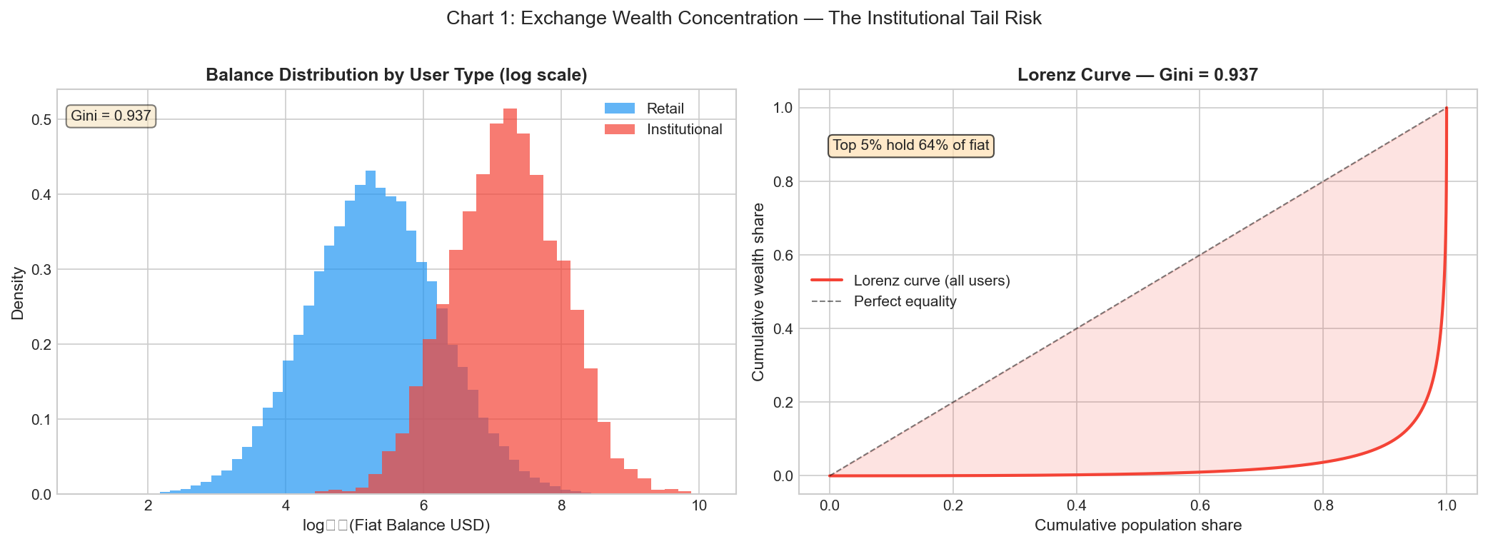
Before modeling withdrawals, the model first maps the user base. The left panel shows the balance distribution for retail and institutional users on a log scale — two distinct populations, separated by roughly two orders of magnitude in average balance. The right panel shows the Lorenz curve for the combined user base: a Gini coefficient of 0.937, with the top 5% of users holding 64% of total fiat on the platform.
This is the empirical foundation for why the model treats retail and institutional withdrawals as two separate processes. An exchange that sizes its reserve against average user behavior is implicitly assuming its user base looks like the left side of the Lorenz curve. It does not.
Chart 2: What the withdrawal tail actually looks like
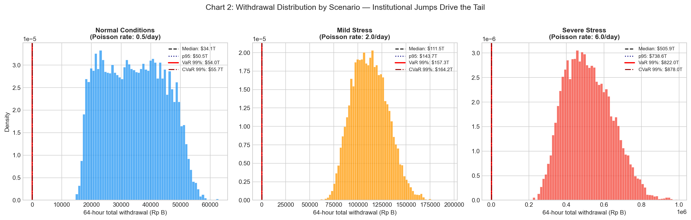
This is the core output of Stage 1 — 10,000 simulated paths per scenario, showing the full distribution of total IDR withdrawals over a 64-hour weekend window.
Under normal conditions, the median weekend withdrawal sits at Rp 34.1T, with the 99th percentile at Rp 54T. Manageable, and consistent with what a standard reserve policy would cover. Under mild stress — a 20–30% crypto drawdown — the median jumps to Rp 111.5T and the tail extends to Rp 164.2T. Under severe stress, the distribution spreads wide: median Rp 505.9T, CVaR 99% at Rp 878T.
The key observation is the shape change, not just the scale. In normal conditions the distribution is tight and roughly symmetric. Under severe stress it becomes flat and heavy-tailed — driven almost entirely by the unpredictable timing and clustering of institutional jump events. A reserve sized for the normal median survives normal weekends. It does not survive the tail.
Chart 4: The reserve level that actually makes a difference
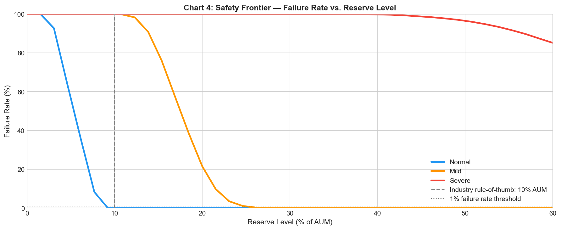
This chart answers the most direct question in reserve policy: if I hold X% of AUM as fiat reserve, what is the probability that it is not enough?
For normal conditions (blue), the answer drops to near zero around 10% AUM — which is also where the industry rule-of-thumb sits (marked by the dashed vertical line). For mild stress (orange), failure rate reaches near zero around 25% AUM. For severe stress (red), the curve barely moves across the entire chart range — still above 85% failure rate at 60% AUM.
The red curve is the critical result. It shows that no practically holdable reserve eliminates tail risk under a severe scenario — which means the right response to severe stress is not a larger reserve alone, but a combination of reserve, credit facilities, and operational escalation procedures. The model quantifies the gap; filling it requires decisions that go beyond treasury policy.
Chart 6: The solvency verdict
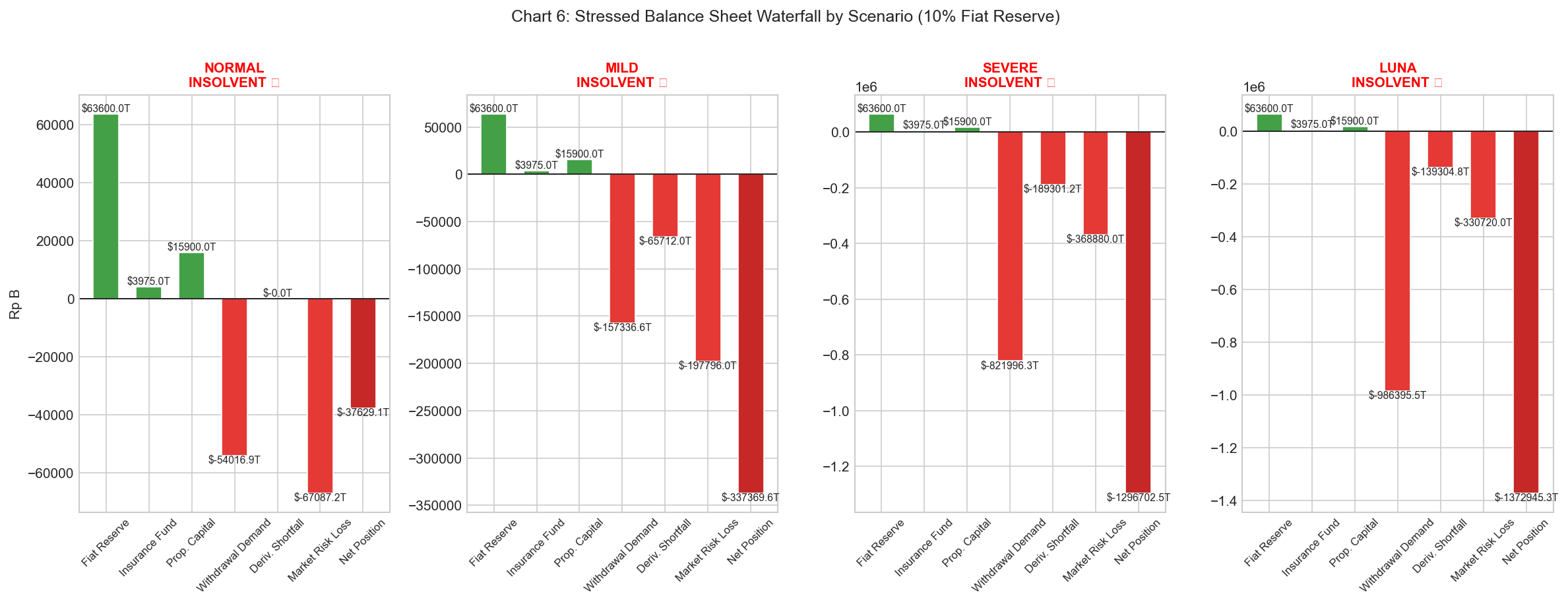
This is where the three dimensions of the model — fiat withdrawal demand, derivatives shortfall, and market risk — are combined into a single stressed balance sheet, tested against a 10% fiat reserve and the OJK regulatory equity floor.
All four scenarios return the same verdict: INSOLVENT. Under normal conditions the net position is -Rp 37.6T. Under LUNA-style stress it reaches -Rp 1,372.9T. The green bars (fiat reserve, insurance fund, proprietary capital) are dwarfed in every scenario by the combined weight of withdrawal demand, derivatives shortfall, and market risk losses.
The point is not that 10% is a reckless reserve — it is an industry-standard one. The point is that standard reserves are sized for average conditions, and the stressed balance sheet makes visible exactly how large the gap is when conditions stop being average. That gap is the number a CFO needs to own, not discover after the fact.
// What it looks like in practice
The interactive dashboard translates the model’s outputs into four operational views — each one designed for a different decision that treasury teams need to make before and during a stress event.
Operational Status gives the at-a-glance picture: current fiat reserve position, insurance fund health, estimated time to reserve exhaustion at current withdrawal velocity, and a weekend readiness verdict. Under the mild stress scenario shown, the dashboard flags institutional lead detected (+3 hours ago), projects exhaustion at hour 23, and issues an immediate escalation notice for a capital gap of -Rp 70.4B. This is the screen operations teams would have open on a Friday evening.
Withdrawal Risk shows the full distribution and cumulative withdrawal paths across all three scenarios. The 64-hour cumulative paths chart makes the divergence visceral: normal and mild stress stay near the reserve line, while severe stress climbs well past it and keeps climbing.
Solvency presents the stressed balance sheet waterfall and the VaR method comparison table — showing how the reserve requirement shifts depending on which method is applied, from Rp 67.1B under historical simulation to Rp 368.9B under a severe direct shock scenario.
Reserve Policy outputs the three-layer allocation recommendation with instrument, size, annual cost, and liquidity profile — and the reserve cost curve showing the optimal holding point between opportunity cost and shortfall risk.
// Regulatory integration summary
The model operationalizes OJK’s POJK No. 27 of 2024 requirements as quantitative constraints rather than qualitative checklists.
| OJK Requirement | Model Implementation |
|---|---|
| Minimum equity Rp 50 billion | Hard solvency floor in stressed balance sheet |
| Max 30% consumer assets in self-custody | Cap on liquidatable crypto buffer (Stage 3) |
| Max 30% of self-custody in hot wallet | Hot wallet ceiling = 9% of total consumer assets |
| 100% consumer fund segregation | Removes pooled consumer IDR from reserve pool |
| Real-time transaction recording | Model inputs assume real-time position data |
// What is not modeled
Institutional herding. The Poisson arrival model assumes each institutional withdrawal decision is independent. In practice, institutional actors observe each other — when one large fund exits, others accelerate. A Hawkes (self-exciting) process would be more accurate. This is a named v2 enhancement.
Multi-currency fiat. IDR reserves do not cover USD demand, which is relevant for exchanges with international users or USD-denominated crypto purchases. A proper multi-currency model requires separate buffer optimization per currency with FX conversion risk. Out of scope for v1.
Rehypothecation. Off-balance-sheet exposure — loans to market makers, pledged collateral — is invisible to this model, as it is to PoR. Requires internal data that is not publicly available.
Cross-exchange contagion. Stress spreads across venues. Modeling network effects requires a multi-entity framework.
Banking service window variation. The model treats the 64-hour weekend window as fixed. In practice, banking availability windows may evolve; the model should be recalibrated if settlement windows expand.
A model that names what it cannot do is more useful than one that does not. All assumptions are documented in assumptions.md in the repository.
// Stack
Python · NumPy · SciPy · Pandas · Matplotlib · Chart.js · HTML/CSS/JS
| Component | Detail |
|---|---|
| Withdrawal simulation | Gamma distribution (retail) + Poisson jump process (institutional) |
| Market risk | Historical simulation + EWMA filtering + Stressed VaR |
| Derivatives | Insurance fund simulation + liquidation cascade (5 iterations) |
| Optimization | Newsvendor framework (analytical) + Monte Carlo validation |
| Regulatory constraints | OJK POJK No. 27/2024 — equity floor, storage ratios, segregation rules |
| Dashboard | Self-contained HTML, data baked in as JS objects |
| Synthetic data | Log-normal user base, regime-switching GBM price history |
Synthetic data only. Does not represent any real entity or exchange. Built by Gilang Fajar Wijayanto — Senior Treasury & Finance Operations